From Vacuum to Voltage: A Reader’s Guide to Electricity
This article began as a ChatGPT Deep Research essay and has been edited and expanded by Adrian Hensler into a combined reading guide and teaching companion.
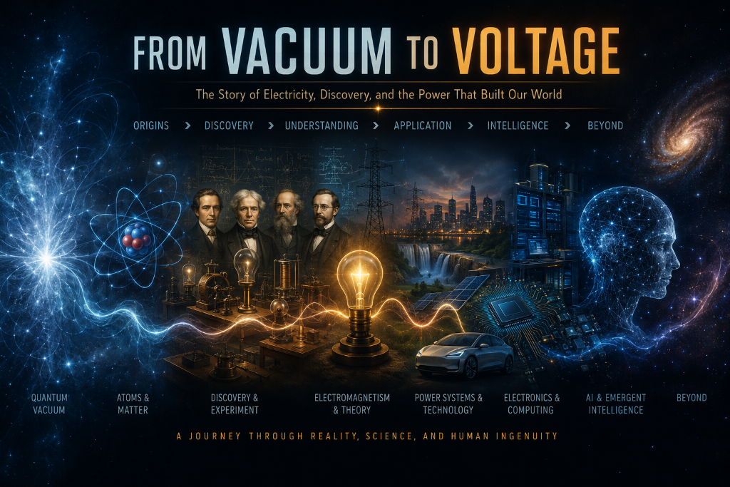
Introduction: One Story, Eight Layers
Electricity is not a separate magical substance. It is one expression of matter, charge, fields, and energy — and understanding it properly means beginning not with a plug socket but with the structure of the universe itself. That is not mysticism. It is the shortest honest path from first principles to the practical question of why lights turn on, why silicon chips work, and why the rise of artificial intelligence is now, unavoidably, a story about power stations and cooling towers as much as algorithms.
This guide follows that path in eight chapters. Each one answers the same layered question at a different altitude: what is actually moving here? What is conserved? What model did earlier thinkers use, and why did a better one eventually replace it? The goal throughout is not to catalogue facts but to track the rhythm of method — the slow, testable, occasionally surprising way that humans narrowed down what electricity really is.
The most important habit to carry through every chapter: each older model you encounter remains useful inside its original domain. Ohm's law still runs the grid. Classical field theory still designs radio antennae. Bohr's atom is still how most people first understand spectral lines. Being replaced by a better model is not the same as being wrong. It means the world turned out to be richer than the earlier version could describe.
This piece works in two modes: first as a long-form narrative about how electricity came to be understood, and then as a practical companion for teaching or self-study, with experiments, measurements, and safety notes.
Chapter 1: The Quantum Vacuum and the Birth of Matter
Where physics can and cannot start
The intellectually honest opening move of any rigorous course on electricity is to say plainly what physics does not know: there is no experimentally confirmed account of what, if anything, existed before the inflationary beginning of the observable universe. That question sits at the edge of current science, not because physicists are incurious, but because the evidence runs out there. The cosmic microwave background, the distribution of galaxies, the abundance of light elements — these all confirm that the observable universe evolved from an extremely hot, dense early state. They do not confirm a literal "before."
What they do support strongly is inflation — a brief period of extraordinarily rapid expansion in the universe's earliest moments. Inflation is currently the leading explanation for why the universe looks so uniform on large scales, and why tiny quantum fluctuations in early fields left imprints that eventually became the seeds of galaxies. This is where the underlying physical framework that eventually permits electricity begins, because those early fields are the same family of entities — quantum fields — that will later express themselves as electrons, photons, and everything else matter does.
The quantum vacuum is not nothing
The phrase "quantum vacuum" is easily misread as meaning "empty space" or even "absolute nothingness." It means neither. In quantum field theory, the vacuum is the lowest-energy state of a set of fields that permeate all of space. It is structured, not featureless. Particles appear in this picture as excitations of those fields — temporary departures from the ground state, like ripples on a pond that has no waves but is still made of water.
A useful image: the quantum vacuum is less like an empty room and more like a perfectly calm ocean. It has structure, rules, and the latent capacity for waves. The absence of waves is not the absence of ocean.
This matters for the story of electricity because the electron — the carrier of electric current in most practical contexts — is one such excitation. It is an excitation of the electron field. The photon, the quantum of light and of electromagnetic radiation, is an excitation of the electromagnetic field. These are not separate inventions. They arise from the same underlying framework, and understanding that framework, even loosely, makes all of the later physics more coherent.
From plasma to atoms: the first few hundred thousand years
After the hot Big Bang, the early universe was a plasma — a state of matter so hot that electrons and nuclei could not combine into stable atoms. Light could not travel freely; it scattered continuously off the charged particles. Then, roughly 380,000 years after the Big Bang, the universe cooled enough for electrons and protons to combine into neutral hydrogen. Light decoupled from matter and streamed outward. That ancient light is what we detect today as the cosmic microwave background, and its tiny temperature variations are the imprint of those early quantum fluctuations.
The formation of neutral atoms was, in a sense, the moment at which chemistry — and eventually electricity — became possible. Once matter could exist in stable neutral configurations, the long story of atomic structure, chemical bonding, conductors, semiconductors, and everything else could begin. The universe had, at that point, been running for less than a million years. The first stars were still hundreds of millions of years away.
Why this matters for understanding electricity
Starting from cosmology is not theatrical. It prevents a specific confusion that haunts many introductions to electricity: the idea that charge, current, and fields are somehow separate from the rest of physics — special phenomena that need their own special language. They are not. They are the macroscopic expressions of quantum field theory applied to matter. The electron is not a mysterious ingredient added to explain electricity. It is the same kind of thing as every other particle, arising from the same underlying structure of the universe. Keeping that in mind makes every later chapter easier.
Chapter 2: Static Electricity — From Amber to Inverse-Square Law
The first observations
Humans noticed electrical effects long before they understood them. The Greek philosopher Thales of Miletus, writing around 600 BCE, observed that rubbed amber attracted light objects. The Greek word for amber is elektron — the etymological root of everything that follows. For roughly two thousand years after Thales, this remained an isolated curiosity rather than a science: an interesting effect, yes, but not a system of ideas that could be tested, extended, or built upon.
The transformation began in 1600, when the English physician William Gilbert published De Magnete, a systematic study of magnetism and, crucially, of what he called the "electric" force. Gilbert was the first to draw a clear distinction between electrical attraction — produced by rubbing many different materials — and magnetic attraction, which he correctly identified as a separate phenomenon. This sounds simple, but it was a genuine intellectual step: it replaced a fog of loosely related curiosities with two distinct, named phenomena that could be studied independently.
Franklin and the concept of charge
Benjamin Franklin's contribution, in the mid-eighteenth century, was to provide electricity with a coherent conceptual framework. Franklin conducted extensive experiments with Leyden jars — early devices for storing charge — and with lightning, famously arguing that lightning rods could protect buildings by offering a conducting path for the electrical discharge. But his deeper contribution was linguistic and conceptual: he introduced the idea of positive and negative charge, and proposed that electrical phenomena could be understood as the movement and redistribution of a single electrical fluid.
Franklin was wrong about the single-fluid model in detail — we now know there are two kinds of charge carrier, not one — but the framework he built was powerful enough to unify a huge range of previously disconnected observations. Lightning, Leyden jars, rubbed glass, electrical sparks: all of them became instances of charge accumulation, transfer, or discharge. That unification is what makes Franklin's work more than a collection of interesting experiments. It was the beginning of electricity as a coherent subject.
Franklin also established the convention that current flows from positive to negative — a convention still used in circuit diagrams today, even though we now know the actual electron flow is in the opposite direction. The convention predates the discovery of the electron by more than a century, and it stuck.
Coulomb and the birth of quantitative electricity
The decisive move toward modern physics came in 1785, when the French engineer and physicist Charles-Augustin de Coulomb measured the force between charged objects using a torsion balance — a device exquisitely sensitive to small forces. His results showed that the force between two point charges varies inversely with the square of the distance between them, and directly with the product of their charges. This is Coulomb's law, and it is the electrical analogue of Newton's law of gravitation.
The cultural shift that Coulomb's work represents is worth pausing over. Before Coulomb, electricity was a subject full of vivid demonstrations and loose theoretical ideas. After Coulomb, it was a subject with a quantitative force law — a mathematical relationship that could be tested, refined, and built upon. The difference between qualitative observation and quantitative law is not merely a matter of precision. A force law allows prediction. It allows engineering. It transforms a curiosity into a tool.
Chapter 3: Current, Voltage, and Resistance — The First Calculable Circuits
From sparks to steady current: Volta's pile
Everything described so far — amber and silk, Leyden jars, lightning rods — involved static electricity: the accumulation of charge that then discharged rapidly and was gone. The transition to continuous electric current required a new device, and it was built in 1800 by the Italian physicist Alessandro Volta.
Volta's invention, the voltaic pile, was built from alternating discs of zinc and silver separated by brine-soaked cloth. The chemical reaction between the metals and the electrolyte produced a continuous flow of charge around an external circuit. Volta had, in effect, invented the battery — not in the modern packaged sense, but in the fundamental sense of a device that could sustain a steady electrical current through an external conductor. This was not merely a laboratory curiosity. It made a whole new set of experiments possible, and it established "current electricity" as a separate subject from the static electricity that Franklin had systematized.
A vivid historical detail: Volta tested some of his early metal combinations on his own tongue, because the instruments of his time were not sensitive enough to detect the small currents his experiments produced. The tongue, connected to the nervous system, is an exquisitely sensitive galvanometer. This is not recommended as a modern practice, but it illustrates how crude the available tools were and how inventive early experimenters had to be.
Ohm and the calculable circuit
The relationship between voltage, current, and resistance was established by Georg Ohm in 1827, in work that was initially received with scepticism but is now foundational to all of electronics. Ohm showed, through careful quantitative measurement, that the current flowing through a conductor is proportional to the voltage applied across it, with the constant of proportionality being what we now call resistance.
This is Ohm's law: voltage equals current multiplied by resistance, or V = IR. It looks almost trivially simple, but its implications are enormous. Circuits become calculable. Given a source voltage and a set of resistances, you can predict the current in every branch. You can design for a desired brightness of a lamp, a desired torque from a motor, a desired signal level in a communication system. Electricity stops being a phenomenon to be observed and becomes a resource to be engineered.
Power: the bridge between electricity and everything else
The other concept that completes the basic circuit toolkit is power — the rate at which electrical energy is transferred or converted. Electrical power is voltage multiplied by current, measured in watts. A 12-volt source driving one ampere of current delivers 12 watts of power. That power might appear as heat in a resistor, as light in a lamp, as mechanical work in a motor, or as radio waves from an antenna. The electrical circuit is just the means of delivering energy from where it is generated to where it is needed.
The relationship P = VI, combined with Ohm's law, gives a complete picture of basic DC circuits. It also gives the first hint of why transmission lines run at high voltage: for a given amount of power to be transferred, doubling the voltage halves the current, and since resistive losses in a wire scale with the square of current, halving the current cuts losses by a factor of four. This principle, which drove the adoption of high-voltage AC transmission in the 1880s and 1890s, follows directly from Ohm's law and the definition of power.
Chapter 4: Magnetism, Induction, and the Reality of Fields
Oersted's compass
The connection between electricity and magnetism was discovered by accident — or nearly so. In 1820, the Danish physicist Hans Christian Ørsted noticed that a compass needle was deflected when placed near a wire carrying electric current. He had been suspecting such a connection might exist, which is why he was watching. But the result was still surprising: a steady electric current produced a steady magnetic effect in the space surrounding the wire, not just at the wire itself.
André-Marie Ampère, working in Paris, heard of Ørsted's result and within weeks had produced a quantitative account of the force between two current-carrying conductors. Ampère showed that parallel currents in the same direction attract each other, parallel currents in opposite directions repel, and the force falls off with distance in a predictable way. Electricity and magnetism, previously separate chapters of natural philosophy, were now demonstrably linked.
Faraday and the crucial insight about change
The next step — arguably the most conceptually important step in the history of classical electromagnetism — was taken by Michael Faraday in 1831. Faraday discovered electromagnetic induction: the fact that a changing magnetic field can drive a current in a nearby circuit, even with no physical contact.
The key word is changing. A steady magnetic field near a wire does nothing. Move the magnet, or switch the current that produces the field on and off, and a current appears in the wire. The induced current is produced not by magnetism per se but by the rate of change of magnetic flux through the circuit. Faraday called the driving quantity the electromotive force, and his law relating it to the rate of flux change is one of Maxwell's four equations.
This is the principle behind every generator and every transformer ever built. A power station generator rotates a coil inside a magnetic field, continuously changing the flux through the coil and thereby continuously inducing a current. A transformer uses a changing current in one coil to produce a changing magnetic field, which induces a current in a second coil — allowing voltage to be stepped up or down without direct electrical contact.
Faraday had no formal mathematical training and developed his ideas almost entirely through physical intuition and experimental craft. He invented the concept of lines of force — the forerunner of what we now call the electromagnetic field — as a way of visualizing how electrical and magnetic effects propagate through space rather than acting instantaneously at a distance.
Maxwell: making the field primary
James Clerk Maxwell gave Faraday's intuitions mathematical form. Between 1861 and 1865, Maxwell assembled the equations of classical electromagnetism into a coherent dynamical theory. The result was four equations — now known as Maxwell's equations — that describe how electric and magnetic fields are created by charges and currents, how they interact with each other, and how they propagate.
The prediction that came out of Maxwell's equations was astonishing: electromagnetic disturbances should propagate through space as waves, and those waves should travel at a speed that Maxwell could calculate from the known constants of electricity and magnetism. The speed he calculated matched the known speed of light to within experimental error. Light is an electromagnetic wave.
This was one of the great unifications in the history of physics. Optics, electricity, and magnetism — three separate subjects — turned out to be aspects of a single phenomenon. And the conceptual move that made it possible was Maxwell's insistence on treating the field — the condition of space around charges and currents — as a physically real entity, not merely a bookkeeping device. The field, not the charged body, is where the physics lives. That reframing echoes all the way forward to quantum field theory.
Chapter 5: The Electron, the Nucleus, and the Quantum Atom
Thomson's discovery and the end of the indivisible atom
By the end of the nineteenth century, the atom was still thought to be the irreducible building block of matter. The word "atom" is from the Greek for indivisible. In 1897, J. J. Thomson ended that idea. Working with cathode rays — streams of particles emitted from a negative electrode in an evacuated tube — Thomson measured the ratio of charge to mass for the particles and showed that they were far lighter than any known atom, and that they were the same regardless of what material the cathode was made from.
Thomson had discovered the electron: a negatively charged particle, much smaller than an atom, present in all matter. The atom was not indivisible after all. It contained smaller pieces. Thomson proposed a model in which electrons were embedded throughout a diffuse blob of positive charge — the so-called "plum pudding" model, in which electrons were the plums suspended in a positively charged pudding.
Rutherford's nucleus
In 1909, Ernest Rutherford, Hans Geiger, and Ernest Marsden performed a series of experiments in which they fired alpha particles — helium nuclei, as it turned out — at a thin sheet of gold foil and measured the angles at which the particles scattered. The plum-pudding model predicted that particles would pass through the diffuse positive charge with only small deflections. What they observed was very different: most particles passed straight through, but a small fraction were deflected at very large angles, and some bounced almost directly backward.
Rutherford later said that this was the most surprising result of his scientific life — "as if you fired a fifteen-inch shell at tissue paper and it came back and hit you." The explanation he arrived at was the nuclear model: atoms are mostly empty space, with a tiny, dense, positively charged nucleus at the centre and electrons distributed somehow in the vast surrounding volume. The plum pudding was wrong. The pudding was gone, and the plums were orbiting an almost point-like core.
The gold foil experiment established a pattern that repeats throughout physics: the most informative experiments are often the ones whose results look at first like they have to be wrong. An unexpected result, rigorously confirmed, is worth more than a hundred expected ones.
Bohr and the quantized atom
Rutherford's nuclear model immediately raised a problem. Classical physics predicted that an electron orbiting a nucleus should continuously radiate energy as electromagnetic waves, spiralling inward and collapsing into the nucleus in a tiny fraction of a second. Atoms are obviously stable, so something was wrong with applying classical physics to this situation.
Niels Bohr, in 1913, proposed a solution that was frankly ad hoc but empirically successful: he simply postulated that electrons could only occupy certain allowed orbits, in which they did not radiate, and that they emitted or absorbed radiation only when jumping between these allowed states. The energy of the emitted or absorbed photon matched the energy difference between the two states. Bohr's model correctly predicted the wavelengths of the hydrogen spectral lines — a precise, quantitative agreement with observation.
Bohr's model was not a complete theory. It worked for hydrogen but failed for more complex atoms, and it left the physical reason for the quantization unexplained. But it established that classical physics could not describe atoms, that something fundamentally new was needed, and that the new theory would have to reproduce the discrete spectral lines that spectroscopes had been measuring for decades.
Schrödinger, wave mechanics, and quantum electrodynamics
The full quantum mechanical account came in 1926, when Erwin Schrödinger developed the wave equation that describes quantum states as wavefunctions — mathematical objects that give the probability of finding a particle at any location. Werner Heisenberg had independently arrived at an equivalent formulation using matrices. The two approaches — wave mechanics and matrix mechanics — were shown to be mathematically equivalent.
In the quantum mechanical picture, an electron in an atom does not have a definite orbit. It has a probability distribution, a cloud of likelihood that encodes where the electron might be found if measured. The allowed energy states emerge naturally from the mathematics of the wave equation, with no need for Bohr's ad hoc quantization postulate. The quantization is built into the physics of waves in a confined region.
A further refinement came with quantum electrodynamics (QED), developed primarily by Richard Feynman, Julian Schwinger, and Sin-Itiro Tomonaga in the late 1940s. QED is the quantum field theory of the electromagnetic interaction — the precise, calculable account of how electrons and photons interact. Its predictions have been verified to more decimal places than any other theory in physics. It is the theoretical foundation on which all of the practical electronics in the following chapters ultimately rests.
Chapter 6: Semiconductors, Transistors, and the Integrated Circuit
Why semiconductors are interesting
The periodic table contains conductors — materials that carry current easily — and insulators — materials that do not. Semiconductors sit between these categories in a way that turns out to be extraordinarily useful. Their conductivity can be controlled: it depends on temperature, on the presence of specific impurities, on applied voltage, on exposure to light. A material whose conductivity can be switched and modulated is the basis of every active electronic device.
The quantum mechanical account of semiconductors uses the concept of energy bands. In a solid, the allowed energy states for electrons form broad ranges — bands — separated by ranges of forbidden energy — gaps. In conductors, the highest occupied band is partially filled, and electrons can move freely within it. In insulators, the gap between the highest filled band and the next empty band is so large that electrons cannot cross it at any practical temperature. In semiconductors, the gap is small enough that a modest input of energy — heat, light, or electric field — can promote electrons across it, creating the conditions for current to flow.
The transistor: a materials breakthrough
The transistor was invented in December 1947 by John Bardeen, Walter Brattain, and William Shockley at Bell Laboratories. It emerged from a sustained research programme into the surface properties of germanium — a semiconductor — and it was from the beginning as much a materials science achievement as a circuit breakthrough. The three inventors received the Nobel Prize in Physics in 1956.
A transistor is, in its simplest description, a device in which a small electrical signal at one terminal controls a much larger current flowing between two other terminals. It can therefore act as an amplifier — a small input producing a proportionally larger output — or as a switch, where the small control signal determines whether a large current flows or is blocked entirely. The switching function is what makes transistors the foundation of digital computing.
Before the transistor, the same switching and amplifying functions were performed by vacuum tubes — glass envelopes containing metal electrodes in a near-vacuum, heated by a filament. Tubes were large, fragile, power-hungry, heat-producing, and finite-lived. A transistor can do the same job in a fraction of the volume, at a fraction of the power, at far greater reliability. The change was not merely incremental. It was what made modern electronics conceivable.
The integrated circuit and the economics of scale
Jack Kilby at Texas Instruments demonstrated the first working integrated circuit in 1958: multiple electronic components — transistors, resistors, capacitors — fabricated together on a single piece of semiconductor material. Robert Noyce at Fairchild Semiconductor independently arrived at a more practical version shortly afterward. Kilby received the Nobel Prize in Physics in 2000; Noyce had died in 1990.
The significance of integration is economic and practical as much as technical. A circuit assembled from discrete components requires that each component be made, tested, shipped, soldered, and connected. Each connection is a potential failure point. Each component occupies physical space and consumes power independently. When all of those components are fabricated together on one crystal, the cost per component drops dramatically, the reliability rises, the physical size shrinks, and the speed increases because signals travel shorter distances.
Gordon Moore, a co-founder of Intel, observed in 1965 that the number of transistors that could be integrated on a chip had been doubling roughly every two years — an observation that became known as Moore's Law. The doubling continued, with some variation, for approximately six decades. A modern high-end processor contains tens of billions of transistors on a chip the size of a fingernail. The transistor density that makes this possible is measured in nanometres — a few dozen atoms across.
Chapter 7: AC, DC, Transformers, and the Electrical Grid
The war of currents
By the 1880s, electricity had moved from the laboratory to the street. Thomas Edison had built the first commercial electric power system in New York in 1882, supplying direct current to customers near his Pearl Street generating station. Direct current is directionally steady: it flows continuously in one direction. Edison's system worked, but it had a serious limitation. Electrical resistance in transmission lines meant that power was lost as heat over distance. To supply customers further away required either thicker (and more expensive) copper cables or generating stations closer together — neither of which was economical at scale.
Nikola Tesla and George Westinghouse championed an alternative: alternating current, which periodically reverses direction. The critical advantage of AC is not that it behaves differently in a wire — it loses energy to resistance in exactly the same way — but that AC voltage can be transformed. A transformer, exploiting Faraday's principle of electromagnetic induction, can efficiently step AC voltage up for transmission and then step it back down for use. Transmitting at high voltage and low current means far lower resistive losses. At the other end, the voltage is stepped back down to safe levels for households and industry.
The eventual adoption of AC was not purely technical. It involved fierce commercial competition, spectacular public demonstrations, and a propaganda campaign by Edison that included electrocuting animals with AC current to demonstrate its supposed danger. The physics eventually won. AC transmission became the world standard, and remains so today.
Frequency and the nature of alternating current
Alternating current in a power system reverses direction at a fixed frequency — 60 hertz in North America, 50 hertz in most of the rest of the world. One hertz means one complete cycle per second: the current rises to its positive peak, falls through zero, reaches its negative peak, and returns to zero, sixty or fifty times every second. The voltage at a wall socket traces a smooth sinusoidal wave in time.
Because AC voltage varies continuously, the concept of "the voltage" at any instant is less useful for engineering purposes than the root-mean-square (RMS) value — a kind of effective average that correctly predicts the power delivered to a resistive load. When a North American electrical system is described as running at 120 volts, that figure is the RMS value. The actual peak voltage is about 170 volts. This distinction matters whenever waveforms and power calculations need to be compared across AC and DC circuits.
Grounding, protection, and the safety architecture of mains electricity
The electrical grid supplies power at voltages that are dangerous to human tissue. The safety architecture of a mains installation is therefore not merely good practice but a system designed around specific failure modes. Understanding it, even conceptually, prevents the most common categories of dangerous error.
In a typical installation, three conductors run to each outlet: line (carrying the alternating voltage), neutral (the return path, nominally at ground potential), and earth ground (a physical connection to the building's earthing system). Earth ground is not normally a current-carrying conductor. It exists to provide a low-resistance path for fault current in the event that a live conductor comes into contact with a metal enclosure or other accessible surface. The fault current trips a breaker or fuse, disconnecting the supply before the fault path through a human body can deliver a dangerous amount of energy.
Ground-fault circuit interrupters (GFCIs) add a further layer of protection by comparing the current in the line and neutral conductors. If those currents differ by more than a small threshold — indicating that some current is taking an unauthorised path, possibly through a person — the GFCI disconnects the supply in milliseconds. This is why GFCIs are required near water sources in most modern electrical codes.
Chapter 8: From Silicon to AI — Computing as an Electrical System
Computation is not abstract
Digital computation is sometimes described as if it were a purely mathematical or logical activity, something that happens in an abstract space of symbols and operations. This description is useful but incomplete. Every logical operation in a computer is implemented as a physical state change in a transistor, and every state change dissipates energy as heat. Memory access moves charge through capacitors. Clock signals drive synchronised switching millions or billions of times per second. The abstraction of software runs entirely on a substrate of electrons, fields, and heat.
This matters because the constraints of the physical substrate are now the central challenges of the most demanding computational workloads. The limits on what AI systems can do are not primarily limits of mathematics or algorithm design. They are limits of power consumption, heat removal, memory bandwidth, and the speed of light across an interconnect. Understanding computing as an electrical system is not a detour around the interesting questions. It is how you get to them.
The architecture of a modern AI accelerator
The dominant hardware for large-scale AI training and inference is the graphics processing unit (GPU), repurposed from its original role in rendering images. A high-end GPU for AI work — Nvidia's H100, for example — contains tens of thousands of small parallel processing cores, a large on-chip cache, and a stack of high-bandwidth memory (HBM) attached directly to the chip package. The H100 can consume up to 700 watts — the power draw of a household appliance — and communicates with its memory at multiple terabytes per second.
The successor H200 increases the HBM capacity to 141 gigabytes and the memory bandwidth to 4.8 terabytes per second. These numbers reveal the central bottleneck of modern AI: not raw arithmetic, but the speed at which data can be fed to the arithmetic units. A modern GPU can perform arithmetic far faster than its memory can supply operands. The performance of an AI workload is frequently limited by memory bandwidth, not by the number of arithmetic operations per second. This is why HBM — memory stacked directly on the processor package — has become the critical component in AI hardware.
From device to rack to datacentre
A single AI training run does not use one accelerator. It uses hundreds or thousands, connected by high-speed network fabric and distributed across racks in a datacentre. The DGX B200 — Nvidia's current AI server — houses eight B200 GPUs with a combined total of 1,440 gigabytes of GPU memory and a maximum power draw of 14.3 kilowatts from six power supply units. This is not a server in the traditional IT sense. It is a significant electrical load requiring dedicated power distribution, liquid cooling, and structural reinforcement.
A rack of traditional IT servers might draw 5 to 10 kilowatts. Industry roadmaps for AI hardware point from current rack densities of roughly 100 kilowatts toward 1 megawatt per rack within a few years. This is not a minor engineering adjustment. It requires fundamentally different approaches to power delivery, cooling infrastructure, and datacentre design.
The grid-level implications are becoming visible in energy planning and infrastructure investment. The International Energy Agency's central projection has datacentre electricity consumption roughly doubling between 2025 and 2030, from around 485 terawatt-hours to around 950 terawatt-hours. Much of that growth is driven by AI workloads. The question of where that electricity comes from — and how reliably and cheaply it can be delivered — is not a technical question in the narrow sense. It is an infrastructure, policy, and investment question that the AI industry cannot answer by itself.
Beyond silicon: the real questions
The limits of silicon-based transistor scaling are real and approaching. Transistor dimensions are now measured in a handful of nanometres, and the physical mechanisms that enable switching — the controlled movement of carriers through a channel — become harder to engineer as the structures shrink toward atomic scale. Leakage current increases. Heat generation becomes harder to manage. The gains in performance-per-watt that drove five decades of Moore's Law are slowing.
Several alternative approaches are under active development. Silicon photonics replaces electrical interconnects with optical ones, addressing the bandwidth-and-power problem for communication within and between chips. Neuromorphic computing attempts to mimic the architecture of biological neural networks, which perform certain computations at extraordinarily low power by using analogue, sparse, event-driven signalling rather than synchronous digital switching. Quantum computing uses quantum mechanical phenomena — superposition and entanglement — to perform certain classes of computation that are intractable for classical machines, though the practical engineering challenges remain formidable.
None of these paths is a guaranteed replacement for silicon, and the field is moving quickly enough that confident long-range predictions are almost certainly wrong in detail. What is not uncertain is the framing: the future of computation is a physics and engineering problem as much as a software one, and the physics begins — as this guide has tried to show throughout — with the structure of matter, the nature of fields, and the behaviour of charge.
Teaching and Lab Companion
What follows expands the essay into a teachable structure, preserving the historical arc while adding practical demos, measurement expectations, and lab discipline.
This course works best as eight modules delivered in sequence, each answering the same systems question from a different altitude: what is really moving, what is conserved, how is it measured, and what changed when a better model arrived?
| Module | Core arc | Practical anchor |
|---|---|---|
| 1 | Quantum vacuum, inflation, hot Big Bang, emergence of matter | Logarithmic timeline and scale-thinking |
| 2 | Static electricity from ancient observation to quantitative charge | Tape, balloon, and electroscope experiments |
| 3 | Volta, Ohm, circuits, voltage, current, resistance, and power | 12 V bench lab with resistor, LED, and multimeter |
| 4 | Ørsted, Ampère, Faraday, Maxwell, induction, and fields | Coil, compass, magnet, and generator demo |
| 5 | Electron, nucleus, spectra, quantum atom, wave mechanics, QED | Spectra demo and model comparison |
| 6 | Semiconductor physics, transistor action, integrated circuits | Diode and transistor switch lab |
| 7 | AC/DC, transformers, grounding, multimeter, oscilloscope | Safe low-voltage AC and ripple measurement |
| 8 | Computing, AI accelerators, datacentre power, future directions | Power-budget and architecture exercise |
Module-by-module teaching notes
Module 1 — From quantum vacuum to the hot Big Bang
Learning objectives: Distinguish quantum vacuum from “nothing”; explain why physics can describe the early observable universe better than a literal pre-origin; use logarithmic scale for time and energy.
Demo: Build a logarithmic timeline across a wall or webpage, with equal spacing for powers of ten from 10-36 seconds to billions of years.
Expected observations: Learners should record powers-of-ten intervals rather than equal-second intervals; the point is scale compression, not stopwatch realism.
Module 2 — Charge, static electricity, and the first electric stories
Learning objectives: Define charge imbalance; distinguish attraction and repulsion from current; understand how early investigators moved from qualitative effects to measurement.
Demo: Use two strips of tape, or a balloon and light paper bits, then add a simple electroscope if available. Charge by friction, test attraction and repulsion, and compare dry and humid conditions.
Expected observations: If an electroscope is available, leaf or needle deflection should increase after charging and decay faster in humid air.
Module 3 — Voltage, current, resistance, and the first calculable circuits
Learning objectives: Explain voltage as potential difference, current as charge-flow rate, resistance as opposition to current, and power as rate of energy transfer; apply Ohm’s law and power relations.
Demo: Build a 12 V isolated bench circuit with a resistor and one LED. Measure source voltage, branch current, resistor drop, and LED drop with a multimeter.
Expected measurements: The voltage drops across the LED and resistor should sum to the source. If a red LED drop is about 2 V and the resistor is 1 kΩ, current should be about 10 mA; halving the resistor roughly doubles the current until component limits intervene.
Module 4 — Magnetism, induction, and field thinking
Learning objectives: Explain the link between current and magnetism; state Faraday’s law qualitatively; relate induction to generators and transformers; understand why Maxwell’s field picture mattered.
Demo: Place a compass near a wire or coil carrying low-voltage DC. Then move a magnet through a coil connected to a meter or scope. Finally, hand-spin a small DC motor as a generator.
Expected measurements: A stationary magnet near a coil produces near-zero steady reading; moving the magnet inward gives a pulse of one polarity and outward gives the opposite. Faster motion or more turns gives larger induced emf.
Module 5 — Electron, nucleus, spectra, and the quantum atom
Learning objectives: Explain what J. J. Thomson, Rutherford, Bohr, and Schrödinger each added; distinguish electron discovery, atomic nucleus, quantized spectra, and wave mechanics.
Demo: Use a diffraction grating to compare a white source with a line-emitting source in a supervised lab, or use a web-based spectral simulator if no tube source is available.
Expected measurements: White sources spread broadly; line-emission sources produce discrete bands; if a hydrogen source is available, a small number of visible Balmer lines should appear at reproducible positions.
Module 6 — Semiconductors, transistor action, and integrated circuits
Learning objectives: Explain why semiconductors are useful; distinguish diode behavior from transistor behavior; understand why the transistor displaced the vacuum tube.
Demo: On the same 12 V bench, measure a diode in forward and reverse direction, then build a transistor switch that turns an LED on with a small base current or gate signal.
Expected measurements: A diode conducts strongly in one direction and poorly in the other within safe limits; a transistor allows a small control input to switch a larger current through the load.
Module 7 — AC, DC, grounding, multimeters, and oscilloscopes
Learning objectives: Distinguish AC from DC; explain why transformers make AC transmission historically dominant; use a multimeter correctly for voltage, resistance, continuity, and current; understand the grounding assumptions of a bench oscilloscope.
Demo: Measure a battery in DC mode, then a low-voltage isolated AC source in AC mode. If available, view the isolated secondary on a scope and compare RMS meter reading with waveform shape. Show ripple after rectification on a safe low-voltage board only.
Expected measurements: The battery should read stable DC; the isolated AC source should show an AC RMS reading; the scope should show time-varying voltage and, after rectification and filtering, visible ripple rather than ideal flat DC.
Module 8 — From chip to AI rack and beyond
Learning objectives: Connect transistor-level switching to modern computing; understand that AI hardware is constrained by power, memory bandwidth, networking, and cooling; identify plausible next directions beyond present silicon scaling.
Demo: Run a power-budget exercise from LED branch to laptop charger to workstation to AI server. If a plug-in power meter is available, measure idle and load on a local computer and compare those readings with official accelerator and server specifications.
Expected measurements: Learners should be able to compute P = VI, convert device-level demand into branch and rack implications, and explain why cooling and interconnect become first-order constraints.
Safety and Instrumentation
All hands-on work in this course should remain inside an isolated low-voltage boundary, preferably 12 V DC for beginner labs. Resistance and continuity measurements belong on de-energized circuits. For fixed wiring, panel work, branch-circuit alterations, and any non-isolated mains work, learners should work only with qualified supervision.
| Tool | First job | First safe habit | First non-obvious trap |
|---|---|---|---|
| Multimeter | Verify voltage, continuity, resistance, current | Check function and jacks before touching the circuit | Measuring resistance on a live circuit |
| Bench supply | Provide known voltage and current limits | Set current limit before connecting the load | Treating a current limit as optional |
| Oscilloscope | See waveform versus time | Connect reference ground deliberately | Assuming the probe ground is a floating magic clip |
| Clamp meter | Non-contact current measurement | Verify CAT rating and conductor placement | Assuming the clamp reading replaces proper voltage safety checks |
AI Hardware as an Electrical System
| Scale | Illustrative figure | Why it matters |
|---|---|---|
| Single accelerator | H100 GPU up to 700 W | Device-level power is already appliance-class |
| Memory-heavy accelerator | H200 with 141 GB HBM3e at 4.8 TB/s | Memory capacity and bandwidth are now central design limits |
| Full AI server | DGX B200 with 8 B200 GPUs, 1,440 GB total GPU memory, 14.4 TB/s NVLink switch bandwidth, and 14.3 kW max input | AI systems are platform-scale electrical loads |
| Rack roadmap | Industry roadmaps point from roughly 100 kW toward 1 MW racks | Power distribution and cooling architecture become strategic constraints |
| Grid consequence | Datacentre electricity demand is projected to rise sharply through 2030 | AI hardware requirements propagate upward into energy policy and grid planning |
Conclusion: The Layered View
The story this guide has told runs from quantum fields at the smallest accessible scale to grid-scale energy infrastructure at the largest. The path is not a detour. Each layer depends on the one below it. The transistor works because of semiconductor band physics. Semiconductor band physics is quantum mechanics applied to periodic crystal lattices. Quantum mechanics replaced classical models that could not explain atomic stability or spectral lines. Those classical models replaced even earlier qualitative accounts that could not explain why amber attracts dust. And the particles that move through all of these structures are excitations of quantum fields that pervade a universe that has been expanding and cooling for nearly fourteen billion years.
The practical upshot is not mysticism. It is this: each layer of the stack generates real constraints that propagate upward. The speed of light limits how quickly information can travel across a chip. Thermal physics limits how densely transistors can be packed. Band structure determines which materials can be semiconductors. Quantum mechanics determines what band structures are possible. None of these constraints are negotiable by software or by faster iteration. They are the physics of the situation, and understanding them is what allows engineers to work intelligently at each layer rather than bumping into walls they did not know were there.
The most important conceptual habit this guide has tried to build is the layered view: the capacity to see any electrical or computational system simultaneously as a physical device, a circuit, a signal-processing system, a power-consuming infrastructure, and an economic object. None of those descriptions is wrong. All of them are necessary. And the ability to shift between them — to ask "what is actually happening in the physics here?" and then "what does that imply for the engineering?" and then "what does that imply for the infrastructure?" — is what separates a deep understanding from a superficial one.
Electricity is not a separate substance. It is matter and charge and fields and energy, all the way down. The vacuum from which it ultimately emerges is not empty. And the voltage in the wire, the current in the transistor, and the rack full of accelerators training a neural network are all chapters in the same long story about what the universe is made of and what we have learned to do with it.